What is Longitudinal data
It is the collection of few observations over time from various sources such a blood pressure measurement during a marathon (1 hour) for many people. It is different from time series data in duration and source. Time series data is collection of lot of observation for one source.
Case Study
install.package("nlme")
library(nlme)
## We will do the analysis on Orthodont Data. It is a study on 27 children (16 boys and 11 girls). Data is the distance of centre of pituitary gland to the pterygomaxillary fissure. There are four measurement at age 8, 10, 12, 14.
head(Orthodont,10)
distance age subject gender
1 26 8 M01 Male
2 25 10 M01 Male
3 29 12 M01 Male
4 31 14 M01 Male
## Questions to answer:
1) Whether distances over time are larger for boys than for girl.
2) Determine whether rate of change of distance over time is similar for boys and girls.
Step 1: Plot(Orthodont)
Step 2:## Create Scatter plot
plot(distance~age, data=Orthodont,
ylab="distance"
xlab="age")
Step 3: ## create scatter plot with smother
with(Orthodont, scatter.smooth(distance, age, col="blue",
ylab="distance", xlab="age", lpars=list(col="red",lwd=3)))

Step 4: fm1<-lmList(distance ~ age | subject, Orthodont)
Step 5: plot(intervals(fm1))

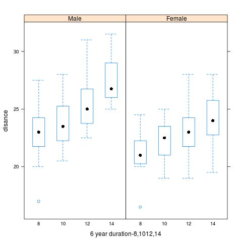
Step 6:## Create Box plot
library(lattice)
bwplot(distance~as.factor(age)|Sex, data=Orthodont,
ylab="Distance",
xlab="6 year duration-8,1012,14")

Analysis:
1) The trajectory of distance is approximately a linear function of age.
2) The trajectories vary between child.
3) The distance measurement increases with age.
4) The distance trajectories for boys are higher on an average than girls.
5) There is a population trend as well as subject specific variation in the data.
It is the collection of few observations over time from various sources such a blood pressure measurement during a marathon (1 hour) for many people. It is different from time series data in duration and source. Time series data is collection of lot of observation for one source.
Case Study
install.package("nlme")
library(nlme)
## We will do the analysis on Orthodont Data. It is a study on 27 children (16 boys and 11 girls). Data is the distance of centre of pituitary gland to the pterygomaxillary fissure. There are four measurement at age 8, 10, 12, 14.
head(Orthodont,10)
distance age subject gender
1 26 8 M01 Male
2 25 10 M01 Male
3 29 12 M01 Male
4 31 14 M01 Male
## Questions to answer:
1) Whether distances over time are larger for boys than for girl.
2) Determine whether rate of change of distance over time is similar for boys and girls.
Step 1: Plot(Orthodont)
Step 2:## Create Scatter plot
plot(distance~age, data=Orthodont,
ylab="distance"
xlab="age")
Step 3: ## create scatter plot with smother
with(Orthodont, scatter.smooth(distance, age, col="blue",
ylab="distance", xlab="age", lpars=list(col="red",lwd=3)))

Step 4: fm1<-lmList(distance ~ age | subject, Orthodont)
Step 5: plot(intervals(fm1))

Step 6:## Create Box plot
library(lattice)
bwplot(distance~as.factor(age)|Sex, data=Orthodont,
ylab="Distance",
xlab="6 year duration-8,1012,14")
Analysis:
1) The trajectory of distance is approximately a linear function of age.
2) The trajectories vary between child.
3) The distance measurement increases with age.
4) The distance trajectories for boys are higher on an average than girls.
5) There is a population trend as well as subject specific variation in the data.

No comments:
Post a Comment